Written by: Karthik Prasad

Calculus is one of the greatest inventions in Mathematics. Its two primary tools—the derivative and integral—allow us to calculate the rates of change and work done respectively,and are used throughout the world. However, it doesn’t always do things the way we need it to, as we’ll explore in the article. To solve these edge cases, mathematicians had to turn to a new kind of integration and a new idea of what it meant to measure a quantity, and through this process, discovered one of the most profound mathematical insights of all time:the Lebesgue Integral. Here, we will discuss what calculus is, where it fails, and how we resolve its shortcomings with measure theory and lebesgue integration. 

Basics of Calculus: Derivatives

In the real world, one of the most common questions we ask is “how fast is something changing?” How fast is your car going, how fast is your debt diminishing, and similar questions are all prevalent in our society, and sometimes, aren’t easy to answer. So, mathematicians attempted to come up with a tool to solve these questions, by noticing that in a line, the rate of change is equal to the slope of the line. So, if we could get a “line” that represents the change of a quantity with respect to another, it’s easy to get the rate of change. This idea was formalized via the idea of limits (the value a function approaches as its input changes value) and the secant and tangent lines, as shown in the following image. 

Figure 1

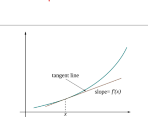
Visual Depiction of the Derivative

Source: Reed College

Basics of Calculus: Integrals

Another very common question is how much of something is there. How much distance have we traveled, how much money have I paid off for my mortgage, and other such questions are all very common, but not easy to answer. This answer is related to the area of a function. This can be seen by thinking about rectangles. When we make 5 dollars per minute, how many dollars do we make in 5 minutes? This is easy: 5 dollars/min times 5 min = 25 dollars.However, these 25 dollars is just the area of the graph of the function b(t) where b(t) is the number of dollars made per time t from t=0 to t=5, since b(t) = 5. Equivalently, the “amount of something” is going to be the area under the graph of the function. Then, if we approximate a complicated function with very small rectangles, then we should be able to get the area of the function and therefore how much work has been done. This gives us the classical Riemann sum, which works well in many cases. However, a finite amount of rectangles will never give us a “perfect approximation” – in Figure 2, for example, the rectangles don’t perfectly approximate the curve. But, if we imagine making every rectangle even smaller and adding more rectangles, we should get an even better approximation. When we take the limit where the length of each rectangle goes to 0 and the number of rectangles goes to infinity, we should get a perfect area.

Figure 2

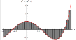
Graphical Depiction of the Riemann Sum Approximation of Area

Source: Graphics by Andrew Charles Jones

Where Riemann Fails

Unfortunately, the Riemann integral doesn’t work everywhere. The best-known example of this is the Dirichlet function. Consider a function where every rational number is equal to 1, and every irrational number is equal to 0. Somewhat intuitively, we expect that there are way way more irrational than rational numbers. So, the contribution of the rationals should basically be ignorable, and then we should just have that the integral (area) of the set is 0, because all the irrationals have value 0. However, the Riemann integral for this function is undefined—it simply isn’t possible to integrate it according to the ways we’ve talked about before. What is the integral of a set? So, we have to think about a different way to integrate.

A New Integral

In a Riemann integral, we start on the x-axis. We’re taking segments of the x-axis, approximating the area with rectangles, and then getting the area of those rectangles. Alternatively,  what if we considered rectangles along the y-axis? Take some segment of the y-axis, and multiply it by “how much x” there is. This is the idea behind the Lebesgue integral, almost “reversing” the Riemann integral. It divides the elements on the y-axis and then finds how much x matches up to them to get a rough measure of how much area there is underneath the overall curve. The issue is, of course, that we don’t know what “how much x” actually is. 

To solve this problem, we introduce the idea of a measure – something that measures “how much x there is”. There are various measures on various sets, but it seems to make sense that the measure of the rationals in the reals is zero – there are a lot more real numbers than rationals. Then, computing the integral of the Dirichlet function is easy – we take all the things with y=0 and all the things with y=1. The y=1 objects have measure 0 (since these are the rationals) so their total contribution to the integral is 0. Therefore, the rest of the integral has area 0 since their y-value is 0, and overall the integral is 0. 

Figure 3

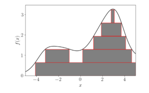
Visualization of the Lebesgue Integral

Source: Graphics by Andrew Charles Jones

Conclusion

We’ve talked about classical calculus and how we can apply similar ideas to more complicated situations, like the Dirichlet function via measures and the Lebesgue integral. This is important because we can treat a greater variety of structures with the Lebesgue integral. For example, it becomes possible to do calculus on complex numbers (a field of mathematics called complex analysis) and other unorthodox structures. The ideas of the Lebesgue Integral and Measure Theory as a field have had revolutionary impacts on mathematics, and all budding scientists should be aware of them. 

References and Sources

Source 1 AXLER, S. (2019). Measure, Integration & Real Analysis. SPRINGER NATURE.

Source  2 Visualizing multivariable functions and their derivative – Project Project. (2017, July 8). https://blogs.reed.edu/projectproject/2017/07/08/visualizing-multivariable-functions-and-their-derivative/

Source 3  Weisstein, E. W. (n.d.). Riemann Sum. Mathworld.wolfram.com. https://mathworld.wolfram.com/RiemannSum.html

Source 4  Jones, A. (2022, March 27). Visualizing Lebesgue integration. Andy Jones. https://andrewcharlesjones.github.io/journal/lebesgue-integral.html