Debunking Flatland: Space Filling Curves
Written by: Gautham Anne
In 1877, George Cantor discovered that the number of points in a 2-dimensional plane is the same as the number of points in a 1-dimensional line. This is tremendously counterintuitive since a plane can have an infinite number of lines placed ‘side by side,’ and stating that one line can pass through every other line seems absurd. Even Cantor himself wrote, “I see it, but I don’t believe it.” This revelation is astounding and has many practical applications. This type of thinking revolutionized the way mathematicians have thought about dimensions and infinitesimal mathematical objects and had transformed the realm of set theory forever.
Rigorous Definitions and More History
Cantor defined a one to one correspondence between the perimeter of a square and the points that lie within it. This means that every point that lies within the square can be mapped, or associated with, a point on the perimeter. This is a common methodology to prove that the cardinality, or the number of elements in a set, of two separate infinite sets are equal. If it can be shown that each element of one infinite set can be associated with exactly one element in another, then the number of elements of both sets must be the same. It is common to call this a bijection between two sets. Thus, sets with a bijective relationship have the same cardinality.
Soon after Cantor’s discovery, a new question arose: “Is there a continuous mapping between a line and a 2 dimensional plane?” In other words, is it possible to trace a line that goes through every point in a plane without lifting the pencil once? After nearly a decade, many different types of such curves were discovered.
Filling Up a Plane with a Curve
There are multiple ways to solve the problem regarding the continuous mapping. For example, two such ‘go-to’ solutions are depicted below, commonly referred to as the ‘lawn mower solutions.’
Figure 1

Lawn Mower Solutions
Source: American Scientist
In 1890, the first successful solution was described by Giuseppe Peano, who was an Italian mathematician also known for his famous Peano Axioms, the set of postulates that all of number theory is based upon. However, Peano did not describe the methodology of creating such a curve, but rather found a mathematical function that defines coordinates x and y given a point t on the line. David Hilbert, often regarded as one of the most influential mathematicians of the 20th century, devised a simple version of Peano’s curve through a recursive, geometrical interpretation. Figure 2 shows the family of Hilbert Curves, through which each iteration, the curve gets closer and closer to reaching a completely filled square. In other words, the limit of the number of points that the curve does not pass through goes to 0 as the iterations increase to infinity.
Figure 2
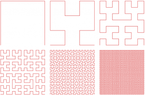
First 6 iterations of the Hilbert Curve
Source: McGill University
Other Space Filling Curves
Although the Hilbert curve is one such mathematical procedure to impose a linear order of points in a 2 dimensional space (linearization), it is not the only one. Mathematicians have discovered numerous different curves which accomplish the same thing, yet have different structures. These curves can be split into recursive space filling curves (RSFC) and non-recursive space filling curves (NRSFC).
Looking at Figure 2, one can determine that each iteration of Hilbert Curves are fractals. That is, the previous iteration is repeated multiple times and joined together to form the next. This is precisely what an RSFC is. Each quadrant of a space RFSC is equivalent to the previous iteration of the curve. NRSFC do not recurse or possess fractal traits. Figure 4 shows some of the most common space filling curves.
Figure 4
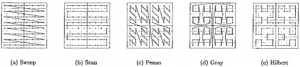
Different types of space filling curves
Source: Purdue University, University of Minnesota
Mathematicians have also generalized space filling curves to any dimension; any multidimensional space can be mapped onto a linear space, or a line. Figure 5 shows some of the common mappings of the 3 dimensional space onto a linear space at an nth iteration.
Figure 5
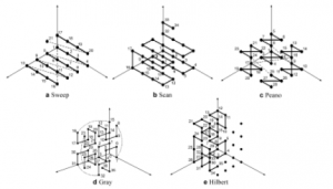
Different types of 3-dimensional space filling curve
Source: Purdue University, University of Minnesota
Locality
One interesting property of some space filling curves is that they preserve locality, which is when a point on the n dimensional space when iterated by a space filling curve does not ‘move’ in the space. The point’s position is as close to being conserved as possible throughout the iterations. The classic Hilbert Curve has remarkable locality preserving properties, and Figure 6 demonstrates this in the 2 dimensional space.
Figure 6
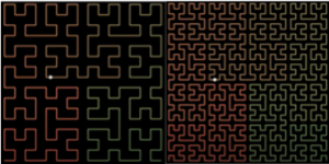
The location of the white point is very nearly preserved throughout the iteration process. This implies that the Hilbert Curve preserves locality very well.
Source: 3Blue1Brown
Applications
Interestingly, many of the properties that space filling curves possess make them very useful for practical applications. One remarkable application of space filling curves was when a couple colleagues at the Georgia Institute of Technology aimed to find efficient routes to deliver meals to elderly clients scattered across Atlanta. This, in principle, is quite similar to the traveling salesman problem, which is notorious in computer science fields. Because some space filling curves preserve locality, a mapping across the streets of Atlanta could be approximated with such curves, providing a close to optimal path, even better than the one that can be predicted from the Bartholdi algorithm.
Another application of space-filling curves is in the realm of linear algebra; specifically, the multiplication of matrices. For a computer to store or read rows and columns of matrices, some values may need to be accessed from the memory multiple times. In 2006, it was found that clustering the data of matrices with space filling curves can reduce memory traffic. Clustering is the process of mapping each cell in an matrix (or in general, an array) to a space filling curve, so the computer only has to store data on a single dimension, similar to how a plane can be mapped to a 1 dimensional line.
Laser printers have also enlisted the assistance of space-filling curves for a process known as half-toning. Half-toning allows laser printers to produce tones of gray. Traditional half-toning uses an array of pixels that vary in size and darkness to produce grays. However, storing the pixels along the path of a Hilbert or Peano curve can help create smoother gradients of gray.
Finally, image processing heavily relies on space filling curves. Originally, each pixel in an image was stored in an array, which required a lot of memory. Later on, it was proposed that each pixel could be mapped onto a Hilbert curve, which would allow every pixel to be represented as a function, rather than an array, thus saving a lot of space. Another advantage of the use of space-filling curves in image processing is that if the resolution of an image changes, the same curve, but a different iteration, can be used since it preserves locality.
Conclusion
From the time of Descartes, it was thought that every point in a d-dimensional space must be represented in d coordinates. For example, in the xy plane, we use two coordinates. However, space-filling curves propose a radically different way of representing multidimensional spaces. A single number can represent every single point, whether that point be in a line, plane, 3 dimensional solid, or even the 11-dimensional spaces that high energy physics involves.
In the novel Flatland, by Edwin Abbott, there exist creatures constrained to a one and two-dimensional world that yearn to break free into higher dimensional spaces. In fact, they might be able to do so, by simply being a space-filling curve.
References and Sources
Crinkly Curves. (2017). Retrieved 19 November 2021, from https://www.americanscientist.org/article/crinkly-curves
Hilbert Space Filling Curves. (2021). Retrieved 19 November 2021, from http://www.bic.mni.mcgill.ca/~mallar/CS-644B/hilbert.html
Mokbel, M., & Aref, W. (2008). Space-Filling Curves. Encyclopedia Of GIS, 1068-1072. doi: 10.1007/978-0-387-35973-1_1233
Space-filling Curve. (2021). Retrieved 19 November 2021, from https://people.math.osu.edu/fiedorowicz.1/math655/Peano.html
(2021). Retrieved 19 November 2021, from https://arxiv.org/pdf/1801.07399.pdf